Factorial and Stirling's approximation

Solving problems by generalization

Expanding the scope of a problem can sometimes be a crucial step in its solution. In mathematics, this pattern translates to expanding the definition of a function or an expression from positive to negative integers, from integers to reals or from real to complex numbers. These generalizations often lead to deep insights and form “bridges” between unconnected areas. We can refer to a couple of ingenious examples of such generalizations:

1. Newton’s generalization of the binomial theorem to negative integers, rational numbers and real numbers

2. Riemann’s generalization of the zeta function to the complex plane

In fact the field of analytic number theory deals with applying methods of analysis (i.e. calculus) to number theory.

It is hard to come up with non-trivial generalizations like the above examples. The study of previously discovered generalizations is therefore a fruitful mental exercise. The aim of this post is to use one such generalization and tinker with the well-known factorial function. Most of the material in this post is available in introductory courses on combinatorics, probability and calculus. While little in this post is new, I hope the content is accessible and amusing. The more rigorous-minded reader can of course find more appropriate resources (Wikipedia as always is a good starting point).

Factorial function

To begin, the factorial of a number $n$ is the result of multiplication of numbers from $1$ through $n$. “$n$ factorial” is denoted by $n!$ and we write:

\[\begin{equation} n! = 1 \times 2 \times \cdots \times n \end{equation}\]

The factorial function belongs to the class of functions called arithmetic functions. As written above, the factorial function is well defined only for positive integers. In applications, the factorial function shows shows up in algorithm complexity theory, combinatorics (arrangements of abstract objects), probability, and statistical physics (arrangements of atoms).

While the mathematical definition of factorial is easy enough to understand, its numerical computation is a different matter. 32- and 64-bit unsigned integers will overflow for $n=13$ and $n=21$ respectively. Most scientific calculators will return floating point answers up to $n=69$. But in real world, we need factorials of numbers much larger than these. In statistical physics, for example, one needs to accurately estimate factorial of $\sim 6\times 10^{23}$ of atoms. How do we go about estimating large factorials?

Generalization of the factorial function

Tasks such as estimating bounds turn out to be easier to perform in the realm of calculus. However, it is not readily apparent how calculus tools can be applied to arithmetic functions and in particular the factorial function defined above. The answer was provided by Daniel Bernoulli in the form of the Gamma function.

Gamma function is defined as

\[\begin{equation} \Gamma(z + 1) = \int_0^\infty x^z e^{-x}dx \label{eq:gamma} \end{equation}\]

The property of the above function is that and for any positive integer $n$, $\Gamma(n + 1)$ equals $n!$.

\[\begin{equation} \Gamma(n + 1) = n! \end{equation}\]

If you’re familiar with integration by parts (from high school or freshman calculus), you can demonstrate this fact quite easily.

It may seem that the Gamma function has made an easy problem unnecessarily complicated. But the opposite is true. Once we generalize an integer-valued problem to real numbers, the latter can be attacked with the full power of calculus. Tools from calculus and analysis allows us to perform not only approximation analysis, but to discover surprising connections to other special functions or entirely different mathematical areas.

In the following we will prove that the factorial of any positive integer $n$ can be accurately approximated by

\[\begin{equation} n! \approx \sqrt{2\pi n}\left(\frac{n}{e}\right)^n \end{equation}\]

and the approximation gets better as n gets bigger. The above approximation to the factorial is known as the Stirling’s approximation. Lets see next how to derive this remarkable formula.

Stirling’s approximation of the factorial

There are a number of ways to derive this formula. Arguably the easiest is to use Laplace’s method. Interested reader may review our brief post on the Laplace’s method. Roughly, the idea in Laplace’s method is this: If you have a function $g(x)$ of the form $g(x) = e^{f(x)}$, and if $f(x)$ has a global maximum at $x = x_0$, then, around $x_0$, $g(x)$ will resemble a Gaussian. Stated differently, if $f(x)$ has a maximum, then, around its maximum, it looks similar to an an inverted parabola and, in turn, $e^{f(x)}$ looks like a Gaussian.

If we’re presented such a $g(x)$, then our task boils down to showing that $f(x)$ has a maximum and to expand $f(x)$ around its maximum to the quadratic term. It turns out that the above trick can be applied to the integrand of the Gamma function.

Let us now work out the details. Consider the integrand in equation $\eqref{eq:gamma}$

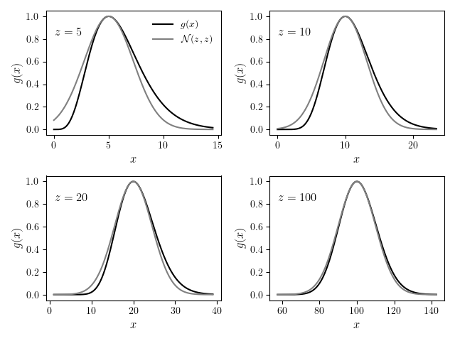
\[\begin{equation} g(x) = x^z e^{-x} \end{equation}\]

Before doing the math, let us understand the behavior of $g(x)$ using intuition and pictures.

$g(x)$ is a combination of two factors $x^z$ and $e^{-x}$. For $z > 0$, the first factor ($x^z$) increases with $x$ and the second factor ($e^{-x}$) decreases with $x$. Thus we should expect $g(x)$ to have a maximum at some value of $x$. When we plot the function $g(x)$ for various values of $z$ we find a maximum as expected. Not only does $A_z(x)$ have a maximum, but for larger and larger values of $z$, $g(x)$ resembles the Gaussian $\mathcal{N}(z, z)$ (i.e a Gaussian distribution centered at $\mu=z$ and having variance $\sigma^2=z$).

Let us now prove informally that the integrand of the gamma function resembles a scaled Gaussian function. To do that we first define

\[\begin{equation} f(x) = \log g(x) = z \log x - x \end{equation}\]

We will now obtain a quadratic expansion for $f(x)$ around its maximum.

\[\begin{align} \begin{split} f'(x) &= \frac{z}{x} - 1 \quad \Rightarrow \quad f(x) \text{ has maximum at } x = z \\ f''(x)\bigg\rvert_{x = z} &= \frac{-z}{x^2}\bigg\rvert_{x = z} =\frac{-1}{z} \end{split} \label{eq:t2} \end{align}\]

Thus our Taylor expansion is, up to the quadratic term

\[\begin{align} \begin{split} f(x) &\approx f(z) + f'(z)(x - z) + \frac{f''(z)}{2}(x-z)^2 \\ &= z \log z - z + 0 - \frac{(x - z)^2}{2z} \end{split} \end{align}\]

This means our integrand of the Gamma function $g(x)$ is

\[\begin{align*} g(x) &= e^{f(x)} \notag \\ &\approx e^{z\log z - z} \,\, e^{-\frac{(x - z)^2}{2 z}} \notag \\ &= \left(\frac{z}{e}\right)^z \,\, e^{-\frac{(x - z)^2}{2 z}} \end{align*}\]

To recap, we have proved that for large $z$’s

The equation above boxed in green is the key simplification which will lead us to the Stirling’s formula. Right hand side of $\eqref{eq:gaussian}$ is precisely the scaled Gaussian function with mean and variance both equal to $z$. The final step is integrating the integrand $g(x)$ to obtain an approximation for $\Gamma(z + 1)$:

\[\begin{align} \begin{split} \Gamma(z + 1) &= \int_0^\infty g(x) dx \\ &= \left(\frac{z}{e}\right)^z \int_0^\infty e^{-\frac{(x - z)^2}{2 z}} dx \\ &= \left(\frac{z}{e}\right)^z \int_{-z}^\infty e^{-\frac{h^2}{2 z}} dh \qquad\ldots\text{putting } h = x - z \\ &\approx \left(\frac{z}{e}\right)^z \int_{-\infty}^{\infty} e^{-\frac{h^2}{2 z}} dh \\ &= \sqrt{2\pi z} \, \left(\frac{z}{e}\right)^z \end{split} \end{align}\]

This completes our informal derivation of the Stirling’s approximation. The $\sqrt{2\pi}$ factor in the approximation gives away the special relationship Stirling’s approximation has to the Gaussian. Stirling’s approximation, in combination with Laplace’s method used in this article can be used to craft a general methods for proving special cases of the Central Limit Theorem. We will take up this fun exercise in another post.

Accuracy of Stirling’s approximation

In this optional section, we examine the accuracy (or equivalently, the speed of convergence) of Stirling’s formula. Notice that we haven’t actually proved that Stirling’s approximation gets better as \(z\) increases.This aspect is a bit more difficult to prove. Most sources just state what is called the Stirling’s series without proof. Stirling’s series indicates that the approximation gets better as $\frac{1}{12 z}$. That is the approximation at $z = 40$ is twice as good as at $z = 20$. Mathematically

\[\begin{equation} \Gamma(z + 1) \approx \sqrt{2\pi z} \, \left(\frac{z}{e}\right)^z\left(1 + \frac{1}{12 z} + O\left (\frac{1}{z^2}\right)\right) \end{equation}\]

To derive the leading correction term, we will use two equations:

\[\begin{align} \begin{split} \Gamma(z+1) &\approx \sqrt{2\pi z} \, \left(\frac{z}{e}\right)^z\\ \Gamma(z+1) &= z\Gamma(z) \end{split} \end{align}\]

Assume that the correction is of the form \(\Gamma(z+1) = \sqrt{2\pi z}(z/e)^z h(z)\) and write

\[\begin{align} z\Gamma(z) &= \Gamma(z+1) \notag \\ z \sqrt{2\pi(z-1)} \frac{(z-1)^{z-1}}{e^z} h(z-1)&= \sqrt{2\pi z}\frac{z^z}{e^z}h(z) \notag \\ e (z-1)^{z - \frac{1}{2}} h(z-1) &= z^{z-\frac{1}{2}} h(z) \notag \\ 1 + z\log\left(1-\frac{1}{z}\right) - \frac{1}{2}\log\left(1-\frac{1}{z}\right) &= q(z) - q(z-1) \label{eq:corr} \end{align}\]

where in the last step we have taken the $\log$ of the previous step and put $q(z) \leftarrow \log h(z)$. We expand $\log (1-\frac{1}{z}) = -\frac{1}{z} - \frac{1}{2z^2} -\frac{1}{3z^3}-\cdots$, recognize that $q(z) - q(z-1) \approx q’(z)$ and simplify equation $\eqref{eq:corr}$ to

\[\begin{align} \begin{split} q'(z) &\approx -\frac{1}{12 z}\\ \Rightarrow q(z) &= \frac{1}{12z}\\ \Rightarrow h(z) = e^{q(z)} &\approx 1 + \frac{1}{12z} \end{split} \end{align}\]

Therefore we arrive at Stirling’s formula with the first order correction term

Written on June 1st , 2021 by Rohan