Approximating the Gaussian with simpler bell curves
Introduction
Can a Gaussian function be approximated with a set of simpler functions? This is the question we’re going to explore in the present article. What exactly is a ‘simpler function’ and why might we want such an approximation? Let us explore these questions first.
To keep things simple, we will restrict ourselves to the simple one dimensional Gaussian function: \(f(x) = e^{-x^2}\). This is the bell curve that most people have good intuition about. It appears often in Statistics and the natural sciences.
The mathematical simplicity of the Gaussian function is deceptive. One area where this becomes apparent is when one tries to compute the total area under the Gaussian curve. For the un-normalized Gaussian function we’re working with, the answer is \(\sqrt{\pi}\). The Gaussian integral seems to be resistant to the standard integration techniques such as \(u\)-substitution and integration by parts.
My original motivation for seeking an expansion of the Gaussian into simpler functions was to tame its integral – I’m always in pursuit of simple ways to evaluate this integral (which equals \(\sqrt{\pi}\)). Once I started on this path, however, this exercise quickly evolved into the more interesting question of how accurately can other bell curves approximate the Gaussian.
With this background in mind, let us provide the problem set up. The first set up is to break down the Gaussian into a series of functions:
\[\begin{equation} e^{-x^2} = f_1(x) + f_2(x) + \cdots + f_M(x) = \sum_{m = 1}^Mf_m(x) \label{eq:gexp} \end{equation}\]If we could express the Gaussian in the above form and if the functions \(f_m(x)\) had closed-form anti-derivatives, then we could obtain interesting series approximations to the Gaussian integral:
\[\begin{equation} \int_{-\infty}^{\infty}e^{-x^2} dx = \sum_{m = 1}^M \int_{-\infty}^{\infty}f_m(x) dx \label{eq:ser} \end{equation}\]The main idea above is quite innocent. However, it turns out that selecting the functions \(f_m(x)\) and evaluating their parameters is tricker than expected. Stay tuned; this exploration will take us through a tour of linear algebra, nonlinear least squares, Gradient Descent and Fourier series.
Choice of the component functions \(f_m(x)\)
Decomposing functions into series of simpler functions is an old and a well understood concept. Two plausible ways to obtain the expansion in Equation \(\eqref{eq:gexp}\) are Taylor expansion and Fourier expansion.
However, our (ostensible) goal is to obtain an approximation for the integral of the Gaussian from \(-\infty\) to \(+\infty\). To achieve this, the series in equation \(\eqref{eq:ser}\) must be integrable term by term. That is, each \(f_m(x)\) needs to be integrable between \(\pm\infty\).
The terms of the Taylor expansion, being polynomials, blow up at \(\pm\infty\). The terms of common Fourier expansions are oscillatory and finite at \(\pm\infty\). They too are not integrable between \(\pm\infty\). 1
For now, we’re convinced that neither Taylor nor the Fourier expansion would work. Even so, the discussion above has provided us with requirements that our component functions \(f_m(x)\) must satisfy in order to be useful for approximating the Gaussian integral:
- Each $\vert f_m(x)\vert$ must decay to zero away from the origin: $\lim_{x\to\pm\infty}\vert f_m(x)\vert \to 0$
- Each $f_m(x)$ must be flat at $x = 0$: $f_m'(0) = 0$
- Each $f_m(x)$ must have a known closed-form integral between $\pm\infty$
Spend a moment to visualize requirements (1) and (2). It will become clear that each \(f_m(x)\) must itself be a bell-like curve. Requirement (3), while not necessary, helps narrow down the choice of possible candidate functions. It is trying to make sure that our problem doesn’t become a purely numerical exercise and that we get interesting series when we plug back \(\int_{-\infty}^{\infty}f_m(x)dx\) in equation \(\eqref{eq:ser}\).
Our original problem can now be viewed as decomposing the Gaussian into simpler bell curves. Before reading further, try and see if you can come up with functional forms for bell curves which satisfy the above requirements.
In theory, functions satisfying the above conditions can be constructed in an infinite number of ways. In practice I found it harder than expected to come up with formulas for bell curves, but eventually stumbled on three alternatives.
The three functional forms belong to rational, exponential, and sinc class of functions. Each class reveals unique and interesting convergence behavior to the Gaussian.
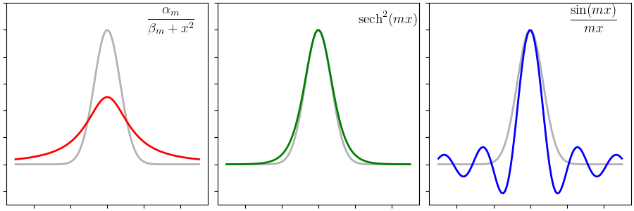
Let us visualize how our three candidate function families look like. The figure below shows the three candidates bell curves overlaid on top of the unnormalized Gaussian function in gray. The rational function, shown first in red, has fatter tails than the Gaussian. The exponential function already seems like a close match and may need only a little tweaking. The sinc function goes below zero and it might be interesting to see how a combination of sincs approaches a Gaussian.
The parametrized form of our three function families can be written as follows:
- Rational function bell curves: $f_m(x) = \frac{\alpha_m}{\beta_m + x^2}$. The expansion looks like $$ e^{-x^2} = \frac{\alpha_1}{\beta_1 + x^2} + \frac{\alpha_2}{\beta_2 + x^2} + \cdots $$
- Exponential function bell curves: $f_m(x) = \alpha_m\,\text{sech}^2(mx)$. The expansion looks like $$ e^{-x^2} = \alpha_1\text{sech}^2(x) + \alpha_2\text{sech}^2(2x) + \cdots $$
- Trigonometric function bell curves: $f_m(x) = \alpha_m\, \frac{\sin(mx)}{mx}$. The expansion looks like $$ e^{-x^2} = \alpha_1\frac{\sin(x)}{x} + \alpha_2\frac{\sin(2x)}{2x} + \cdots $$
It is easy to check that each of the proposed \(f_m(x)\) satisfy conditions (1), (2) and (3) above.
Note that the expansions in terms of our proposed functions \(f_m(x)\) are not guaranteed. Just because we formally wrote the expansion does not imply that it will hold. We have not shown the set of functions \(f_m(x)\) to be complete. Hence there are no theoretical guarantees that the above expansions will converge to Gaussian.
Intuitively however, it must be possible to express the Gaussian as a combination of other bell curves. But how do we choose the parameters of \(f_m(x)\) that give the best possible approximation to the Gaussian function? Had we used the Taylor or Fourier expansions, we could have obtained closed-form formulas for the coefficients \(\alpha_m\) and \(\beta_m\). Without any theory, we will be forced to use a fitting procedure.
The coefficients \(\alpha_m\) and \(\beta_m\) will therefore be determined using the least squares fit of the right-hand side (RHS) expansion with the left-hand side (LHS) function.
The quality of the fit
The quality of a fit is typically measured using the \(R^2\) metric. The \(R^2\) metric tells us how well the formula approximates the given data on a point-by-point basis. The values of the parameters are not usually relevant and do not feature in an \(R^2\) calculation.
For our current problem though, the coefficients do mean something. In fact, the coefficients are bound by a conservation law (or, alternatively, and invariance condition) that depends on the form of \(f_m(x)\). To see this, we can carry out the integration in equation \(\eqref{eq:ser}\) (reproduced below)
\[\begin{equation} \int_{-\infty}^{\infty}e^{-x^2} dx = \sum_{m = 1}^M \int_{-\infty}^{\infty}f_m(x) dx \end{equation}\]The LHS is known to be \(\sqrt{\pi}\) and the RHS is also known for our three candidate \(f_m(x)\):
\[\begin{equation} \int_{-\infty}^{\infty}f_m(x) dx = \begin{cases} \frac{\pi\alpha_m}{\sqrt{\beta_m}} &\qquad \text{ for } f_m(x) = \frac{\alpha_m}{\beta_m + x^2} \\[0.1in] \frac{2\alpha_m}{m} &\qquad \text{ for } f_m(x) = \alpha_m\,\text{sech}^2(mx) \\[0.1in] \frac{\pi\alpha_m}{m} &\qquad \text{ for } f_m(x) = \alpha_m\,\frac{\sin(mx)}{mx} \end{cases} \end{equation}\]This leads to the invariance conditions for the coefficients as follows
The boxed equations above express a remarkable fact: regardless of the numerical value of individual coefficients, they are, as a group, bounded by the conservation condition. This fact is not deep. It is obvious from the formal series expansion in equation \(\eqref{eq:ser}\). But it contrasts with experience we typically have with least-squares regression. In a typical least-squares fit, the coefficients are free to assume any value. Here we are trying to approximate a well-known function. So the coefficients have extra constraints.
These constraints help us formulate a more interesting way to measure convergence. Once the fit is computed, we will measure its quality not by its \(R^2\) but by how well the computed coefficients approximate \(\sqrt{\pi}\). The LHS of equations \(\eqref{eq:cc1}\), \(\eqref{eq:cc2}\) and \(\eqref{eq:cc3}\) express this convergence in simpler terms. That is, we simply have to see how close the LHS approaches $1.0$ rather than having to remember \(\sqrt{\pi}\).
Computing the fit
The fitting procedure is implemented using a simple Gradient Descent approach. The section at the end of this post provides the mathematical formulation and its implementation from scratch in Python.
Approximation using rational functions
We start our study with a small value of \(M\). The fit gives us the coefficients which we can use to write the approximation explicitly. For \(M = 3\) the Gradient Descent fit gives the reasonable (but uninspiring) approximation:
\[\begin{equation} e^{-x^2} \approx \frac{2.0188}{1.2006 + x^2} + \frac{0.4473}{1.1776 + x^2} - \frac{3.0000}{2.9089 + x^2} \end{equation}\]The invariance condition is also satisfied approximately:
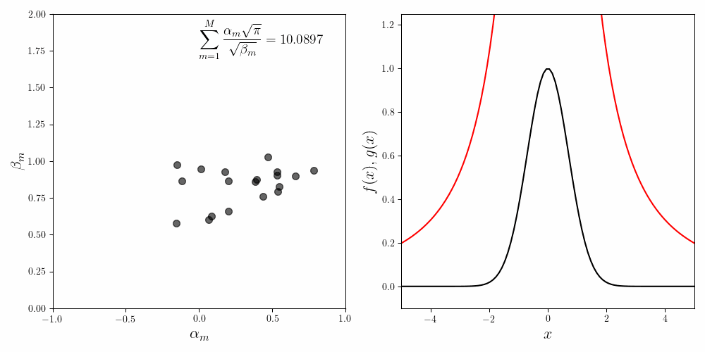
\[\begin{equation} \frac{2.0188\sqrt{\pi}}{\sqrt{1.2006}} + \frac{0.4473\sqrt{\pi}}{\sqrt{1.1776}} - \frac{3.0000\sqrt{\pi}}{\sqrt{2.9089}} \approx 0.87 \end{equation}\]To improve the fit we have to increase the number of component functions. We can bump up to \(M=20\). The figure below shows the convergence of the fitting procedure. The coefficients start with random initial values. As the Gradient Descent iterations progress, the coefficients converge to their final values. Their trajectories look cool, but have no identifiable pattern.
In the inset we show the invariance condition. As the fit converges, the invariance condition \(\sum_{m=1}^M\frac{\alpha_m\sqrt{\pi}}{\sqrt{\beta_m}}\) approaches $1.0$. Due to the nature of the approximation the final value is close to $0.92$ in stead of $1.0$.
The right hand side shows how the quality of the final fit the Gaussian obtained using $20$ component functions \(f_m (x)\). One of the things to realize is that the tails of a Gaussian decay faster than any polynomial. It is quite hard to approximate this fall off using rational polynomial functions like we have chosen. This fact is obvious when we look closely at the quality of the fit at the tails.
Also, the coefficients seem to ‘run away’ as the fitted curve approaches the Gaussian. This is classic overfitting.
Solutions are not unique !
Even for a fixed value of \(M\), the values as well as the orbits of the fitting coefficients vary wildly. The figure below shows three successive runs of the fitting procedure for \(M=20\). In all three cases the fit is decent. The invariance condition is also obeyed with reasonable accuracy. Yet the values and the trajectories of the coefficients are noticeably different in all three cases.
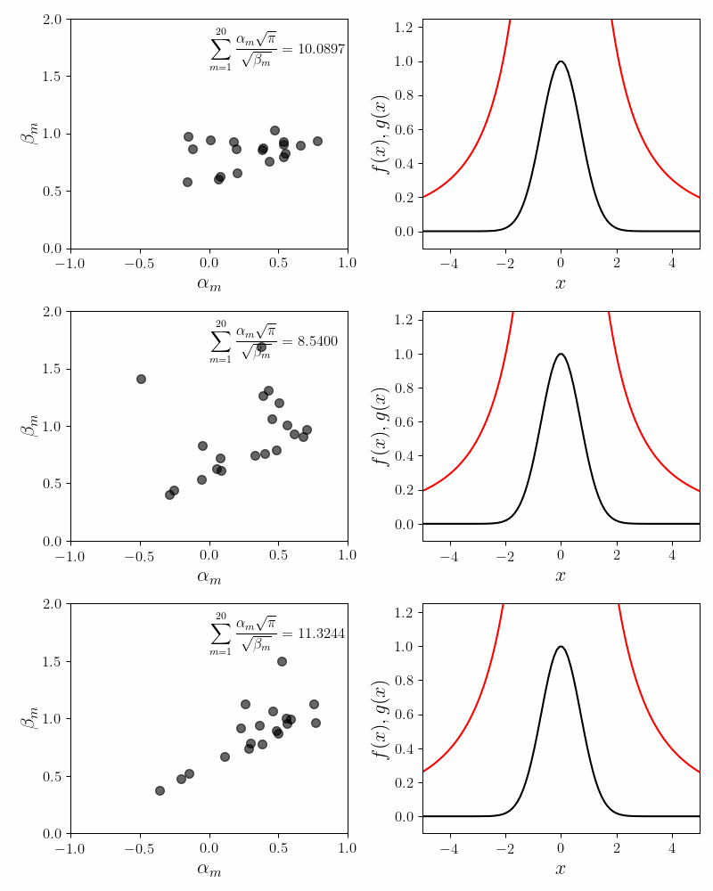
In ML parlence, our problem has multiple minima of comparable qualities. We suffer from the multiple minima problem for two reasons. First, fitting Cauchy-like functions (alternatively known as Lorentzian curves) is always problematic. Even for a single function \(f_m(x) = \frac{\alpha_m}{\beta_m + x^2}\), many values of \(\alpha_m\) and \(\beta_m\) can evaluate to the same function value.
Second, our component functions are degenerate. That is, for a fixed \(\beta\) we can obtain a given function value as \(\frac{0.2}{\beta + x^2} + \frac{0.8}{\beta + x^2}\) or as \(\frac{0.6}{\beta + x^2} + \frac{0.4}{\beta + x^2}\). Thus we should expect a lot of degenerate solutions. The cure for the degeneracy is to somehow distinguish (or unique-ify) the component functions \(f_m(x)\). This is one line of work we’re pursuing currently.
Presently, the multiple minima problem unfortunately prevents us from exploiting any structure in the coefficients. The procedure in this post will be practically useful only if we could determine \(\alpha_m\) and \(\beta_m\) without any elaborate fitting procedure. If we’re able to obtain unique solution, then perhaps we can obtain interesting identities we originally sought.
More component functions = more accuracy
Despite the issues mentioned above, one aspect is consistent with our intuition. Our fits become more accurate with more component functions. The plot below shows the fits for \(M = 8\), \(20\) and \(64\) component functions.
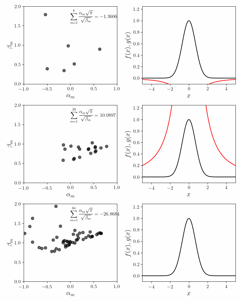
Our proxy for accuracy is the quality of the invariance condition. For $8$, $20$ and $64$ component functions, the value of the invariance sum equals $0.90$, $0.92$ and $0.95$.
Another interesting fact is that as we add more component functions, the coefficients cloud becomes stiffer. The coefficients \(\alpha_m\) and \(\beta_m\) have to travel less distance to achieve an accurate fit. For smaller values of \(M\), the coefficients have to travel a bit further to obtain an accurate fit. This is an observational fact and I do not have intuition for why this might be.
Approximation using exponential functions
Next, let us see how the exponential family of functions approximate the Gaussian. The exponential function family we have chosen is \(\text{sech}^2(mx)\). Recall that \(\text{sech}(x) = \frac{2}{e^{x} + e^{-x}}\). Exponential functions decay faster than rational functions. On the surface, therefore, exponential functions should have an easier time approximating the rapid decay of the tails of the Gaussian.
Formally, the approximation of the Gaussian using a sum of \(\text{sech}^2\) functions is expressed as:
\[e^{-x^2} = \sum_{m=1}^{M}\alpha_m \text{sech}^2 (mx)\]Note that we only have a single parameter \(\alpha_m\) to fit. So the parameter plots here will be one-dimensional. As before, the coefficients \(\alpha_m\) are obtained using Gradient Descent. The animations below show how the partial sums with $M = 8, 16, 32\, \text{and } 64$ approximate the Gaussian.
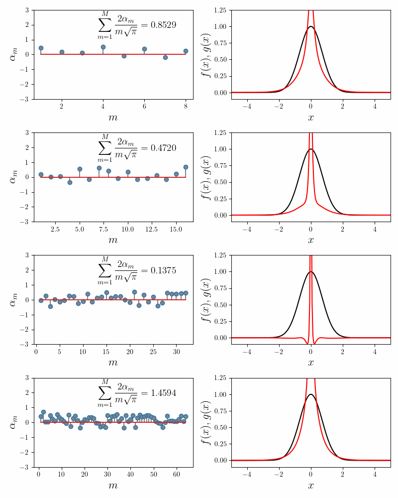
The general observations made for rational functions apply here as well. Because the tails of \(\text{sech}^2(x)\) decay slower than the Gaussian, overfitting, as evidenced by wildly swinging coefficients, is needed to obtain a good numerical accuracy. Adding more component functions provides a more flexibility; for a given accuracy, the coefficients for \(M=64\) swing a lot less than those for \(M=8\).
Approximation using sinc functions
This is the familiar sinc function. In fact the sinc function looks like the Gaussian around \(x = 0\). But it has wiggles and dips below zero. It will be interesting to see how well we can approximate the Gaussian using a ‘sum of sincs’.
Our formal series expansion of the Gaussian in terms of sinc functions will be
\[\begin{equation} e^{-x^2} = \sum_{m=1}^M\alpha_m \frac{\sin(mx)}{mx} \label{eq:exp} \end{equation}\]Note that our component functions are now distinguished. This means that we need precise amounts of the component functions to construct our Gaussian. Because \(\sin(mx)\) and \(\sin(nx)\) have different frequencies, deficiencies from \(f_{m}(x)\) cannot be offset by \(f_n(x)\). This was not true for rational functions \(f_m(x) = \frac{\alpha_m}{\beta_m + x^2}\); a slight decrease in \(\alpha_m\) here could be offset by equal increase in \(\alpha_n\). This led to degeneracy (non-unique solutions) and we hope our new component functions will lead to unique expansion coefficients (turns out to be true).
We first try the fit using \(M=8\) component functions. In the figure below, the left panel shows how the coefficients \(\alpha_m\) converge to their final values. The inset to the left panel shows the value of the invariance condition. With \(M = 8\) component functions, we have about \(6\%\) error. The right panel compares the approximated function (in red) to the Gaussian function (in black).
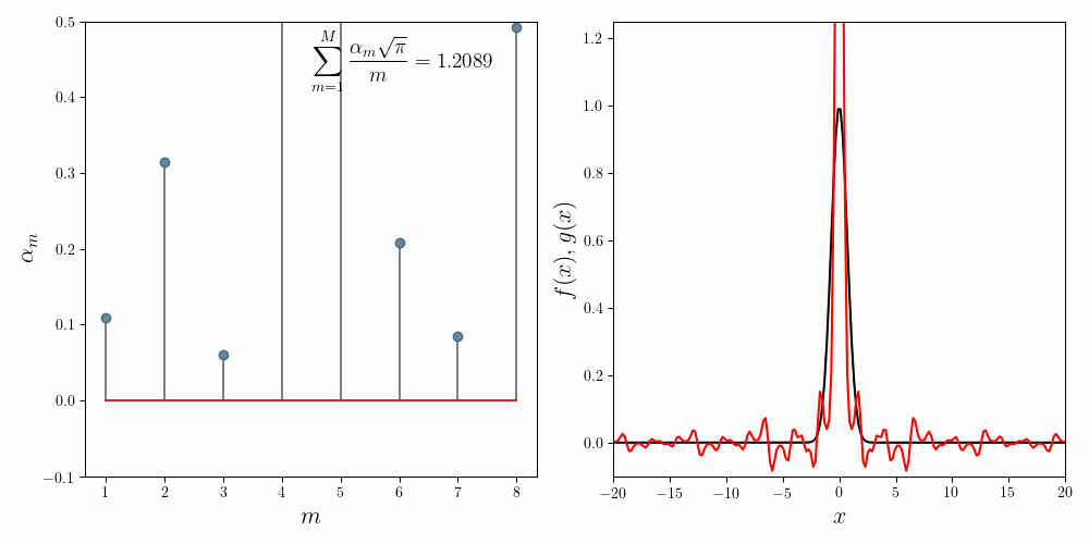
The explicit expansion with the first five terms looks like
\[e^{-x^2} \approx 0.2091\frac{\sin(x)}{x} + 0.4090\frac{\sin(2x)}{2x} + 0.2767 \frac{\sin(3x)}{3x} + 0.0895\frac{\sin(4x)}{4x} + 0.0149\frac{\sin(5x)}{5x} + \cdots\]Repeated runs with different random initializations converge to the same coefficients. This confirms our main hypothesis that the expansion using the sum of sincs is non-degenerate.
Notice that while the main lobe of the Gaussian is quite well approximated by the sum of sincs, there are decaying but visible blips at $x = \pm k\pi$. Increasing the number of component functions does not help. In fact the coefficients \(\alpha_m\) after \(m = 5\) decay exponentially to $0$. The following figure confirms this.
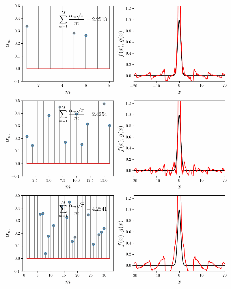
The error in the invariance condition (i.e. the fit quality) also does not dip below $6\%$ regardless of the number of component functions chosen. There are two possibilities as to why the fit isn’t better. It is either our implementation of Gradient Descent procedure, or the form of our components functions. Let us dive deeper into it.
The problem is linear
For the sinc function expansion, we can perform least-squares regression without Gradient Descent. An observant reader might have noticed that with sinc component functions, the problem reduces to ordinary linear least squares (OLS) in disguise. To see that, we will rewrite equation \(\eqref{eq:exp}\) as follows. At any given point \(x_i\) we have
\[e^{-x_i^2} = \alpha_1\frac{\sin(x_i)}{x_i} + \alpha_2\frac{\sin(2x_i)}{2x_i} + \alpha_3 \frac{\sin(3x_i)}{3x_i} + \cdots\]which is of the form
\[y_i = \alpha_1 z_{1i} + \alpha_2 z_{2i} + \alpha_3 z_{3i} + \cdots\]Thus, for all points \(x_i\) we can form the matrix equation
\[\begin{equation} y = Z\alpha \label{eq:neq1} \end{equation}\]where \(y\) is the column vector of Gaussian function evaluated at all values \(x_i\), \(\alpha\) is the column vector of unknown expansion coefficients and \(Z\) is the design matrix. Equation \(\eqref{eq:neq1}\) are simply the normal equations of an OLS problem with the solution
\[\begin{equation} \alpha = \left(Z^TZ\right)^{-1}Z^Ty \end{equation}\]The normal equations can be implemented straightforwardly in Python
def _fit_sinc_linear_regression(x, num_base_functions):
    M = num_base_functions
    x = np.clip(x, 1e-6, None)
    mvals = np.arange(1, M + 1, dtype=float).reshape(-1, 1)
    mx = (mvals * x).T
    Z = np.sin(mx) / mx
    y = np.exp(-x * x)
    ztz = Z.T @ Z
    zty = Z.T @ y
    alphas = np.linalg.inv(ztz) @ zty
    return alphas
We get good agreement between the expansion coefficients computed using the normal equations and Gradient Descent. The numerical comparison between Gradient Descent and normal equations is given below.
| Coefficient | Gradient descent | Normal equations |
|---|---|---|
| \(\alpha_1\) | $0.209173$ | $0.209172559$ |
| \(\alpha_2\) | $0.4090211$ | $0.409018987$ |
| \(\alpha_3\) | $0.276756$ | $0.276752323$ |
| \(\alpha_4\) | $0.0895346$ | $0.089527342$ |
| \(\alpha_5\) | $0.0148756$ | $0.014865627$ |
| \(\sum_{m=1}^5\frac{\alpha_m\sqrt{\pi}}{m}\) | $0.9420$ | $0.9420$ |
This is a comforting sanity check on our Gradient Descent implementation. But it doesn’t really shed light on why our error is stuck at $6\%$ and why the coefficients decay rapidly down to zero for \(m > 5\). For that we need an analytical understanding of the problem.
Analytical solution
Up until now, we tried to find the expansion coefficients \(\alpha_m\) using regression methods. The advantage of the regression methods is that they are general. However, the fitting procedure does not explain the behavior of the regression coefficients; we have to accept them as is. In the present instance we do not know why components after the first five sinc functions do not have appreciable coefficients.
One of the remarkable things about this problem is that it is possible to analytically calculate the expansion coefficients. I stumbled on this solution accidentaly and don’t know if there exists a general theory of function decomposition in terms of non-orthogonal, non-complete basis functions.
Starting from the definition of the expansion
\[e^{-x^2} = \sum_{m=1}^M\alpha_m\frac{\sin(mx)}{mx}\]we multiply both sides of the equation by \(\cos(kx)\) and integrate between \(\pm\infty\)
\[\begin{align} \begin{split} \int_{-\infty}^{\infty}e^{-x^2}\cos(kx)dx &= \sum_{m=1}^M\alpha_m\frac{\sin(mx)\cos(kx)}{mx}\\[0.1in]\ \sqrt{\pi}e^{-k^2/4} &= \sum_{m=1}^M\frac{\pi\alpha_m}{2m}\left[\text{sgn}(m + k) + \text{sgn}(m - k)\right] \end{split} \label{eq:sgn} \end{align}\]We have $M$ undetermined coefficients and have one such equation for each value of $m$. Now the signum is $1$, $0$ or $-1$ depending on whether its argument is positive, zero or negative. So the term inside the square brackets on the right side of equation \(\eqref{eq:sgn}\) will assume the following values
\[\begin{equation} \left[\text{sgn}(m + k) + \text{sgn}(m - k)\right] = \begin{cases} 2 & m > k \\[0.1in] 1 & m = k \\[0.1in] 0 & m < k \end{cases} \end{equation}\]This allows us to write out the expanded form of equation \(\eqref{eq:sgn}\) as
\[\begin{alignat*}{5} \frac{e^{-1^2/4}}{\sqrt{\pi}} &= \frac{\alpha_1}{2\cdot 1} &+ \frac{\alpha_2}{2} &+ \frac{\alpha_3}{3} &+ \cdots &+ \frac{\alpha_M}{M} \\ \frac{e^{-2^2/4}}{\sqrt{\pi}} &= &\frac{\alpha_2}{2\cdot 2} &+ \frac{\alpha_3}{3} &+ \cdots &+ \frac{\alpha_M}{M} \\ \frac{e^{-3^2/4}}{\sqrt{\pi}} &= &&\frac{\alpha_3}{2\cdot 3} &+ \cdots &+ \frac{\alpha_M}{M} \\ \vdots\\ \frac{e^{-M^2/4}}{\sqrt{\pi}} &= &&&&\,\frac{\alpha_M}{2\cdot M} \end{alignat*}\]In the matrix form we have
\[\begin{bmatrix} \frac{e^{-1^2/4}}{\sqrt{\pi}}\\ \frac{e^{-2^2/4}}{\sqrt{\pi}}\\ \frac{e^{-3^2/4}}{\sqrt{\pi}}\\ \vdots \\ \frac{e^{-M^2/4}}{\sqrt{\pi}} \end{bmatrix} = \begin{bmatrix} \frac{1}{2\cdot 1}& \frac{1}{2} & \frac{1}{3} &\cdots &\frac{1}{M} \\ 0 & \frac{1}{2\cdot 2} & \frac{1}{3} &\cdots &\frac{1}{M} \\ 0 & 0 & \frac{1}{2\cdot 3} &\cdots &\frac{1}{M} \\ \vdots \\ 0 & 0 & 0 &\cdots &\frac{1}{2\cdot M} \end{bmatrix} \begin{bmatrix} \alpha_1\\ \alpha_2\\ \alpha_3\\ \vdots\\ \alpha_M \end{bmatrix}\]This is a linear system of equations expressed in matrix notation as
\[\begin{equation} b = U\alpha \label{eq:triu} \end{equation}\]Here, we should pause and take a note of one fact. If we were dealing with a regular Fourier Transform, the matrix $U$ would be a pure diagonal matrix, giving us explicit formula for each individual Fourier coefficient. Here, though, we have an upper triangular matrix. So while we have Fourier-like decomposition, we dont get a nice formula for individual coefficients. Instead we get a system of equations whose solution yields the desired coefficients.
The system of equations \(\eqref{eq:triu}\) can be solved efficiently by using the fact that we have an upper triangular matrix. We basically start by solving the last equation and substitute the solution in the next-to-last equation and propagate upward. The Python code for the solution of the equation system is below
import numpy as np
from scipy.linalg import solve_triangular

def _fit_sinc_analytical(num_base_functions):
    M = num_base_functions
    q = np.arange(1, M + 1, dtype=float)

    # Construct b
    b = np.exp(-q * q / 4) / np.sqrt(np.pi)

    # Construct U
    v = 1. / q
    U = np.tile(v, (M, 1))
    U = np.triu(U, 0)
    E = np.ones((M, M))
    np.fill_diagonal(E, 0.5)
    U *= E

    # Now solve the upper triangular system
    alphas = solve_triangular(U, b, lower=False)
    return alphas
Surprisingly, the analytical solution yields different value of expansion coefficients than the one obtained from regression. The analytical coefficients also yield vastly more accurate approximation to $\sqrt{\pi}$ than the coefficients obtained by regression.
| Coefficient | Analytical | Normal equations |
|---|---|---|
| \(\alpha_1\) | $0.249182799$ | $0.209172559$ |
| \(\alpha_2\) | $0.428984565$ | $0.409018987$ |
| \(\alpha_3\) | $0.245054777$ | $0.276752323$ |
| \(\alpha_4\) | $0.066313512$ | $0.089527342$ |
| \(\alpha_5\) | $0.009551615$ | $0.014865627$ |
| \(\sum_{m=1}^5\frac{\alpha_m\sqrt{\pi}}{m}\) | $0.9996$ | $0.9420$ |
Optional: Gradient descent implementation
This section is a bit mathematical and is optional for those unfamiliar as well as very familiar with machine learning (ML)! The mathematical details are presented here primarily for my own notes and secondarily as an illustration of how to set up a complete ML computation from scratch.
From an ML perspective, we have a nonlinear least squares fitting problem (NLLS) on our hand. The Gauss-Newton method is perhaps the ideal choice for its solution. But we will instead go down an easier route of implementing a simple Gradient Descent fitting algorithm.
The Gradient Descent is implemented in the standard way. We discretize \(e^{-x^2}\) using \(N\) points on the $x$-axis. At each point \(x_i\), we compute the squared residual between the actual function value and the estimated function value. Finally we sum up all \(N\) residuals to obtain the total loss function.
We will keep the presentation general by retaining \(f_m(x)\) for the $m$th component function and use specific forms of $f_m(x)$ only when we need the final formulas.
\[\begin{equation} L = \sum_{i=1}^{N}\left(e^{-x_i^2} - \sum_{m=1}^M f_m(x)\right)^2 \end{equation}\]The second step is to compute the derivative of \(L\) with respect to the parameters:
We can obtain explicit formulas for the gradients by substituting the exact form of \(f_m(x)\). For example, for \(f_m(x) = \frac{\alpha_m} {\beta_m + x^2}\) we have:
\[\begin{align} \frac{\partial L}{\partial\alpha_m} &= \sum_{i=1}^{N} \frac{-2}{\beta_m + x_i^2} \left(e^{-x_i^2} - \sum_{m=1}^M \frac{\alpha_m}{\beta_m + x_i^2}\right) \\[0.2in] \frac{\partial L}{\partial\beta_m} &= \sum_{i=1}^{N} \frac{2\alpha_m}{\left(\beta_m + x_i^2\right)^2} \left(e^{-x_i^2} - \sum_{m=1}^M \frac{\alpha_m}{\beta_m + x_i^2}\right) \end{align}\]The final step is the implementation of the Gradient Descent update equations.
\[\begin{align} \alpha_m &\leftarrow \alpha_m - \eta\frac{\partial L}{\partial\alpha_m} \\[0.1in] \beta_m &\leftarrow \beta_m - \eta\frac{\partial L}{\partial\beta_m} \end{align}\]where $\eta$ is the learning rate. The Python implementation of the three steps is simpler than their mathematical appearence. The code snippet below shows the essence of the implementation for the case of \(f_m(x) = \frac{\alpha_m} {\beta_m + x^2}\). Analogous math and code can be written for the \(\text{sech}^2\) and sinc expansions. The complete code can be found in our Github.
def compute_fit(x, num_base_functions, niters,
                learning_rate, regularization_param):
    M = num_base_functions
    reg = regularization_param
    alphas = np.random.random((M, 1))
    betas = np.random.random((M, 1))

    for t in range(niters):
        v1 = alphas / (betas + x * x)
        r = np.exp(-x * x) - v1.sum(axis=0)
        q = betas + x * x
        v3 = -2.0 / q * r
        v4 = (2.0 * alphas) / (q * q) * r
        dla = v3.sum(axis=1).reshape(-1, 1)
        dlb = v4.sum(axis=1).reshape(-1, 1)
        alphas -= learning_rate * dla
        betas -= learning_rate * dlb

    return alphas, betas
Footnotes
-
An interesting side question is this:
must the Fourier basis functions always be oscillatory and of finite magnitude at \(\pm\infty\)?
The answer is no; there are many examples of orthonormal basis functions that decay to zero at infinity. In fact, the wave functions of Quantum Mechanical bound states are guaranteed to form an orthonormal basis and decay to zero at \(\pm\infty\). The eigenfunctions of the one-dimensional quantum harmonic oscillator or Airy functions are some examples.
Unfortunately, these bound state wave functions do not have elementary anti-derivatives, which is one of our requirements. An interesting follow-up question then is:
can we construct Hermitian operators whose eigenfunctions have elementary anti-derivatives? More generally, given an orthonormal basis function set, can we construct the corresponding potential well function for the Schrodinger equation?