Introduction to Calculus of Variations

Calculus of variations (COV) sits in the gap between calculus and optimization. In regular calculus, we learn to find max or min of functions. COV is not about finding optimal values for a given function but about finding a whole function that optimize a given objective. This is a higher-level goal and is what makes the subject both challenging and useful.

Let us illustrate with a simple example. A maxima/minima problem in regular calculus might ask us to find a point $x$ where the function $f(x) = x^2 e^{-2x}$ achieves its max or min value. To solve this, we calculate $f’(x)$ using rules of differential calculus and set $f’(x) = 0$ to find the desired $x$.

A typical problem in COV will ask us to find a function $y = f(x)$ that maximizes the area bounded by $f(x)$ while holding its perimeter constant. Or a shape that minimizes the distance between two fixed points. A bit of pondering will convince you that such problems cannot be solved by regular calculus alone. What should we differentiate and set to zero to find an entire function? Some piece seems missing.

There is, however, a branch of regular calculus that concerns itself with calculating whole functions: Differential Equations. If we could somehow get differential equations for these optimization problems, we could find the function that satisfies our requirements. COV provides these differential equations.

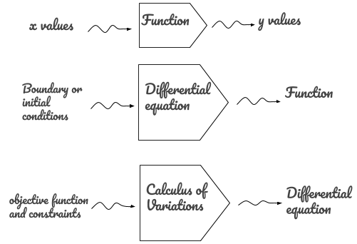
Loosely speaking, COV is a final piece in a progression of widgets. Functions accept values and output values; the parameters of the functions are hardcoded. Differential equations accept boundary conditions and output functions; parameters of the differential equation are hardcoded. Equations of COV accept an objective function (plus any constraints) and output differential equations; parameters of the objective function are hardcoded. The picture below helps visualize the hierarchy.

Once we note that most of our fundamental physical laws are expressed as (partial) differential equations, we can immediately recognize that COV is essentially a machine for crunching laws. Of course, the law will ever be only as good as the objctive function we feed to the machine.

In many fields, however, the objective functions turn out to be easier to guess than the new laws. This probably has to do with the fact that our laws are expressed in terms of partial differential equations describing vector fields. We as humans, on the other hand, inherently lack ability to imagine vector fields and multidimensional spaces. COV provides tools to derive vector laws from scalar objective functions. The importance of this aspect is hard to overstate. In addition, there is more uniformity in the structure of objective functions than there is in the laws they generate.

It is worth seeing briefly how COV game is played in different fields before moving to the examples.

Connections to other fields

In Physics, there is an important toolbox called the minimization principles (also known as Variational Principles). A popular (and successful) technique in theoretical Physics can be described as follows. We start by expressing a known law of Physics (e.g. Newtonian mechanics) in terms of a minimization principle (Lagrangian mechanics). This reformulation has the same physical content as the old theory and by itself it does not produce new laws. However, it leads us to new mathematical structures for the old theory that is more ‘higher level’ or abstract. Then there is a leap of faith. It is hypothesized that this mathematical structure is obeyed not only in the known-and-old field (e.g Newtonian mechanics) but also in new-and-unknown fields (e.g. Quantum Field Theory). Once this is accepted, the game is then to guess the right quantity to minimize and use the techniques of COV to find a new law of Physics. Considerable insight is required to guess the right minimization objective and a coming up with these often represents life’s work for some theoretical physicists. Experiment, of course, is the final judge of whether the guess was right or wrong. A good summary of well-known minimization principles in Physics can be found on Wikipedia.

Minimization principles also play an important role in computational Physics. If a suitable minimization principle is known for a problem, it enables computational solutions to otherwise difficult-to-handle problems. Calculation of the energy levels of Helium atoms is an elementary example of a variational technique applied to a theoretically difficult computation. Taken to its logical extreme by including more particles and interactions, this leads to a powerful framework of Density Functional Theory for calculating crystal structure of solids. Such calculations are the starting point for creating materials with desired thermal, mechanical, chemical and electronic properties. These engineered materials form the backbone of the technology needed for addressing pressing challenges such as climate change and space-exploration.

Motivation for use of variational techniques (and by extension COV) is more straightforward to understand in Artificial Intelligence and Machine Learning. Many algorithms in these fields directly depend on finding functions that minimize certain quantities (e.g. regularized loss functions). In addition to vanilla optimization, there are techniques that are specifically inspired by energy minimization principles. Energy minimization for image segmentation or stereo depth estimation can be cited an examples.

Standard form of the COV problem

Hopefully the above examples have provided a broad sense of why COV and the variational techniques what it begets are fundamental to a lot of fields. In the remainder of this post, we will get gently introduced to COV. First we will overview the fundamental equation of COV–the Euler-Lagrange equation. We will then see how to apply this equation by solving two classic problems step-by-step. Nothing more than a knowledge of regular college calculus will be needed to understand the material.

The two problems we will solve are the isoperimetric problem and the max-entropy problem. While these problems are solved in most textbooks on the subject, it is extremely helpful to internalize the concepts by going over them by ourselves.

As said earlier, the standard minimization problems is to find the $x_0$ which minimizes a given scalar function $f (x)$. By a scalar function we mean a function that returns a scalar value. The input variable $x$ can be a scalar or a vector. The minimization problem in COV is to find the $f(x)$ which minimizes the objective function $J[f]$. An objective function is also known as a functional, or simply a ‘widget that consumes functions’. A functional is not unlike higher-order functions in some programming languages. To reiterate, a regular function $f$ takes an input $x$ and outputs a scalar $y$. A functional takes the whole function $f$ and outputs a scalar. We can write the action of a functional in symbols as follows:

\[\begin{equation*} J[f] = \text{a scalar value} \end{equation*}\]

Any subroutine which calculates the mean, median, variance, or area, of an input function is a functional. Objective functions used in machine learning algorithms are functionals. There are examples of functionals in scientific libraries (e.g. numerical integration using Simpson’s rule). Fourier transform, on the other hand, is not a functional by our definition since it takes in a function and outputs another function, not a scalar.

For COV problems we cannot write a general recipe like solve $f’(x) = 0$ since finding an $f(x)$ that minimizes $J[f(x)]$ is a harder problem than finding an $x$ that minimizes $f(x)$. We therefore have to proceed by identifying special cases of $J[f]$ and tailoring equations for them. The most common special case is one where $J$ depends on the integral of a function $L()$ which is itself a function only of $x$, $y =f(x)$ and $y’= f’(x)$. That is

\[\begin{equation*} J[y] = \int L(x, y, y')dx \end{equation*}\]

While this may seem like a oddly specific form, it turns out that a variety of optimization problems can be expressed in the above form or its extensions. An important point to note is that the function $L$ can encode our optimization objective as well as the constraints.

The Euler-Lagrange equation

Once the optimization problem is expressed in the above form, and the $L$ function is derived, the next step is to form a differential equation for $y = f(x)$. The differential equation for $y$ is obtained from $L$ function via the famous Euler-Lagrange equation:

\[\begin{equation} \label{eq:el} \boxed{\frac{\partial L}{\partial y} = \frac{d}{dx}\frac{\partial L}{\partial y'}} \end{equation}\]

In computing the derivatives of $L$, we treat $y$ and $y’$ as independent variables. That is, when computing $\partial L/\partial y$ we do not worry about derivative of $y’$ with respect to $y$. Similarly when computing $\partial L/\partial y’$ we do not worry about derivative of $y$ with respect to $y’$. If we perform the manipulations in equation \eqref{eq:el}, it yields a differential equation in terms of $x$, $y$ and $y’$. In the final step we solve the differential equation to obtain $y(x)$, the shape (or function) that was originally sought. This is the part about COV being a machine for generating differential equations that, when solved, produce functions which satisfy our original objective.

To add constraints, we use a the method of Lagrange multipliers. This method modifies the $L(x, y, y’)$ function using the constraints and allows us to still use the Euler-Lagrange equations. The method of Lagrange multipliers will become clear when we work with examples.

What we just did was gloss over a huge subject in three short paragraphs. Yes it makes me uncomfortable too. However, instead of worrying about the details left out, our approach for now is to focus on using the above as a recipe: Given an optimization objective and constraints:

1. Construct an $L$ function in terms of $x$, $y$ and $y’$ (assuming its possible)

2. Use the Euler-Lagrange equation to get a differential equation for $y$ and

3. Solve the differential equation for $y$ to get the actual curve.

Once this process is familiar and trusted, it becomes easier to appreciate the theory behind the Euler-Lagrange equations. Now lets test how the recipe works on a couple of classic problems.

Isoperimetric problem

The isoperimetric problem can be stated as follows:

determine a plane figure of the largest possible area whose boundary has a specified length.

In other words, we’re given a loop of an inelastic wire of perimeter $S$ and asked for a shape $y = f(x)$ that will maximize the area $A$ of the shape. I’ve asked this question to dozens of people between the ages of 10 and 80 and almost everyone has given a correct answer (circle). Yet it is a nontrivial matter to actually prove that the intuitive answer is indeed the right one.

As stated above, our three-step recipe is to (1) derive an appropriate $L$ function for the problem, (2) use the Euler-Lagrange equation to get a differential equation for the curve and (3) solve the differential equation to get the actual shape.

We can use well-known formulas for the area $A$ and the perimeter $S$ of a planar curve:

\[\begin{align*} & A = \int y dx \\ & S = \int \sqrt{1 + y'^2} dx \end{align*}\]

These formulas allow the following mathematical statement of the isoperimetric problem:

\[\begin{align*} \text{maximize}&\qquad \int y dx \\ \text{subject to}&\qquad \int \sqrt{1 + y'^2} dx - P = 0 \end{align*}\]

Using the method of Lagrange multipliers, we can convert this into

\[\begin{equation*} \text{maximize}\qquad J[y] = \int \left(y - \lambda \sqrt{1 + y'^2} \right) dx, \end{equation*}\]

where we have ignored the constant term $\lambda P$ since it wont survive the derivatives in the Euler-Lagrange equations. This is the standard form if we identify

\[\begin{equation*} L(x, y, y') = y - \lambda \sqrt{1 + y'^2} \end{equation*}\]

which gives us the $L$ function we were after. Plugging into the Euler-Lagrange equation we obtain

\[\begin{align*} \frac{\partial L}{\partial y} &= \frac{d}{dx}\frac{\partial L}{\partial y'} \\ \Rightarrow 1 &= \lambda \frac{d}{dx} \frac{y'}{\sqrt{1 + y'^2}} \\ \Rightarrow \frac{x + h}{\lambda} &= \frac{y'}{\sqrt{1 + y'^2}}\\ \Rightarrow y' = \frac{dy}{dx} &= \frac{\pm(x + h)}{\sqrt{\lambda^2 - (x+h)^2}} \end{align*}\]

This is a simple differential equation, whose solution

\[\begin{equation*} (x + h)^2 + (y + k)^2 = \lambda^2 \end{equation*}\]

is the standard equation of a circle centered at $(-h, -k)$ and radius $\lambda$.

Max entropy problem

The max entropy problem is simpler calculus-wise but involves multiple constraints in a single problem. One version of the max entropy reads:

Among all probability distributions $p(x)$ of known mean $\mu$ and known variance $\sigma^2$ find the one with largest entropy.

Entropy of a (continuous) random variable $X$ with PDF $p(x)$ is given by $H = -\int p(x)\log p(x) dx$. The entropy is our optimization objective and the known mean, variance and probability normalization condition are our constraints for this problem. As before, we can express the problem mathematically as

\[\begin{align*} \text{maximize}&\qquad \int -p(x)\, \log p(x)\, dx \\ \text{subject to}&\qquad \int p(x)\, dx = 1 \qquad \ldots \text{normalization}\\ &\qquad \int x\, p(x)\, dx = \mu \qquad \ldots \text{known mean}\\ &\qquad \int x^2\, p(x)\, dx = \sigma^2 + \mu^2 \qquad \ldots \text{known variance} \end{align*}\]

Using the recipe for Lagrange multipliers we can transform the above optimization problem with constraints into the standard form:

\[\begin{equation*} J[p] = \int L(x, p, p') dx \end{equation*}\]

where

\[\begin{equation*} L(x, p, p') = -p \log p - \lambda_1 p - \lambda_2 xp -\lambda_3 x^2p \end{equation*}\]

The derivatives of $L$ with respect to $p$ and $p’$ are

\[\begin{align*} \frac{\partial L}{\partial p} &= -1 - \log p -\lambda_1 - \lambda_2 x -\lambda_3 x^2\\ \\ \frac{\partial L}{\partial p'} &= 0 \end{align*}\]

Substituting into Euler-Lagrange equation we get

\[\begin{align*} -\log p &= 1 + \lambda_1 + \lambda_2 x + \lambda_3 x^2 \\ \\ \Rightarrow p(x) &= A e^{-(a x + b x^2)} \end{align*}\]

where $A = e^{-(1+\lambda_1)}$, $a = \lambda_2$ and $b = \lambda_3$. Notice that in this case the differential equation we obtained reduced to a simple algebraic one. To proceed further we use the standard integrals for a Gaussian function (e.g. from Wolfram Alpha)

\[\begin{align*} \int p(x)\, dx &= A\, \sqrt{\frac{\pi}{b}} e^{a^2/4b} = 1 \\ \int x\,p(x)\, dx &= A\, \sqrt{\frac{\pi}{b}} e^{a^2/4b} \left(\frac{-a}{2b}\right) = \mu \\ \int x^2\,p(x)\, dx &= A\, \sqrt{\frac{\pi}{b}} e^{a^2/4b} \left(\frac{a^2}{4b^2} + \frac{1}{2b}\right) = \mu^2 + \sigma^2 \end{align*}\]

The above equations allow us to write the undetermined constants $A$, $a$ and $b$ in terms of given quantities $\mu$ and $\sigma$ as

\[\begin{equation} \label{eq:coeffs} A = \sqrt{b/\pi}e^{-a^2/4b}, \qquad \mu = -a/(2b), \qquad \sigma^2 = 1/(2b) \end{equation}\]

With these equations, $p(x)$ can be written as

\[\begin{equation*} p(x) = \sqrt{\frac{b}{\pi}}\, e^{-a^2/4b}\, e^{-(ax + bx^2)} = \sqrt{\frac{b}{\pi}}\, e^{-b(x + \frac{a}{2b})^2} \end{equation*}\]

Finally substituting the coefficients $a$ and $b$ from equation \eqref{eq:coeffs} we get

\[\begin{equation*} p(x) = \frac{1}{\sqrt{2\pi\sigma^2}} \, e^{-\frac{(x-\mu)^2}{2\sigma^2}} \end{equation*}\]

which is a normal distribution with mean $\mu$ and variance $\sigma^2$.

Generalizations of Euler-Lagrange equations

The two problems we solved so far used the $L$ function that depended on $x$, $y$ and $y’$. There are many generalizations of $L$ functions. Three practically important generalizations that immediately follow the one we’ve considered are the following.

1. $L(x, y, y’, y’’)$:

   The $L$ function depends on a single function of a single variable, but the dependence involves higher order derivatives. This case could arise in variational problems involving curvature. The Euler-Lagrange equation for this case has a second derivative term:

   \[\begin{equation*} \frac{\partial L}{\partial y} - \frac{d}{dx}\frac{\partial L}{\partial y'} +\frac{d^2}{dx^2}\frac{\partial L}{\partial y''} = 0 \end{equation*}\]

2. $L(t, f(t), g(t), f’(t), g’(t))$:

   The $L$ function depends on two functions $f$ and $g$, both of which depend on a single variable $t$. This case arise for a variational problem defined on a parametric curve. In this case we get two coupled first order Euler-Lagrange equations:

   \[\begin{align*} \frac{\partial L}{\partial f} = \frac{d}{dt}\frac{\partial L}{\partial f'} \\ \\ \frac{\partial L}{\partial g} = \frac{d}{dt}\frac{\partial L}{\partial g'} \end{align*}\]

3. $L(x, y, z(x, y), z_x, z_y)$:

   The $L$ function depends on a function of two variables $z(x, y)$ and their first derivatives. This case could arise for variational problems in higher dimensions. E.g. isoperimetric problem for a sphere. In this case the Euler-Lagrange equation has a term that looks like total derivative:

   \[\begin{equation*} \frac{\partial L}{\partial z} = \frac{\partial}{\partial x}\frac{\partial L}{\partial z_x} + \frac{\partial}{\partial y}\frac{\partial L}{\partial z_y} \end{equation*}\]

Further generalization are possible and the reader is referred to Wikipedia for more.

Isoperimetric problem revisited

We will explore generalization #2 in more detail using the isoperimetric problem again. Instead of directly seeking the function $y(x)$ we will parametrize the $x$ and the $y$ coordinates using a single dependent variable $t$ and using two functions: $x = x(t)$ and $y = y(t)$. To derive the new $L$ function, we need the formulas for the area and the perimeter of this parametrized curve. To that end we will consider two successive points along this curve separated by an infinitesimal distance $\Delta t$. The situation is depicted in the figure below.

The area of this infinitesimal triangle is

\[\begin{align*} \Delta A &= \frac{1}{2} \begin{vmatrix} 0 & 0 & 1 \\ x(t) & y(t) & 1 \\ x(t + \Delta t) & y(t + \Delta t) & 1 \end{vmatrix} \\ &= \frac{1}{2}\left[ x(t) y(t + \Delta t) - y(t) x(t + \Delta t)\right] \\ &= \frac{1}{2}[x(t) y'(t) - y(t) x'(t)]\Delta t \qquad\ldots \text{using } f(t + \Delta t) \approx f(t) + f'(t)\Delta t \\ dA &= \frac{1}{2}(x y' - x'y)dt \qquad \ldots \text{differential notation} \end{align*}\]

The total area $A$ enclosed by the curve is the sum over areas of all infinitesimal triangles as the parameter $t$ is varied over its range: $A = \int \frac{1}{2}(x y’ - x’ y) dt$.

The perimeter $\Delta s$ of the exterior segment of the infinitesimal triangle is

\[\begin{align*} \Delta s^2 &= (x(t+\Delta t) - x(t))^2 + (y(t+\Delta t) - y(t))^2 \\ &= (x'(t)^2 + y'(t)^2)\Delta t^2\\ ds &= \sqrt{x'^2 + y'^2} dt \qquad \ldots \text{differential notation} \end{align*}\]

The total perimeter $S$ is the sum of lengths of all such segments: $S = \int \sqrt{x’^2 + y’^2}dt$.

With the total area and total perimeter in hand, the $L$ function for our constrained optimization problem in the parametrized coordinates can be written as

\[\begin{equation*} L(t, x, y, x', y') = \frac{1}{2}(xy' - x'y) + \lambda \sqrt{x'^2 + y'^2} \end{equation*}\]

As mentioned before, we have two sets of Euler-Lagrange equations, one each for $x$ and $y$. From the $x$ equation we get

\[\begin{align*} \frac{\partial L}{\partial x} = \frac{d}{dt} \frac{\partial L}{\partial x'} & \Rightarrow y' = \lambda \frac{d}{dt} \frac{x'}{\sqrt{x'^2 + y'^2}} \\ \\ \frac{\partial L}{\partial y} = \frac{d}{dt} \frac{\partial L}{\partial y'} & \Rightarrow -x' = \lambda \frac{d}{dt} \frac{y'}{\sqrt{x'^2 + y'^2}} \notag \\ \end{align*}\]

These are two coupled, second-order ordinary differential equations. One easy way to solve these is to first integrate the left sides of both equations to obtain:

\[\begin{align} \frac{(y + k)}{\lambda} &= \frac{x'}{\sqrt{x'^2 + y'^2}} \label{eq:elx} \\ \frac{-(x + h)}{\lambda} &= \frac{y'}{\sqrt{x'^2 + y'^2}} \label{eq:ely} \end{align}\]

and then dividing equation \eqref{eq:ely} by equation \eqref{eq:elx} to get

\[\begin{align*} \frac{y'}{x'} &= \frac{dy}{dx} = \frac{-(x + h)}{y + k} \end{align*}\]

which is a single first-order equation, whose solution

\[\begin{equation*} \Rightarrow (x + h)^2 + (y + k)^2 = C \end{equation*}\]

is once again the standard equation of a circle.

Summary

We dipped our toes in the fascinating world of calculus of variations. We stated the fundamental equation of COV, the Euler-Lagrange equation, and saw a few of its generalizations. Though we didnt delve into it, the form of the Euler-Lagrange equations has deeper significance and it makes recurring appearances in Physics and Optimization.

We next saw how to construct the $L$ function and solve the Euler-Lagrange equations for a couple of standard examples. As a result, we can now prove how circle is the shape that maximizes the area of a loop of given perimeter. Hopefully this modest exercise has provided you some appreciation for COV and left you with a sense of curiosity for further exploration.

Written on August 11th, 2020 by Rohan